Introduction to Classification & Regression Trees (CART)

Decision Trees are commonly used in data mining with the objective of creating a model that predicts the value of a target (or dependent variable) based on the values of several input (or independent variables).  In today's post, we discuss the CART decision tree methodology.  The CART or Classification & Regression Trees methodology was introduced in 1984 by Leo Breiman, Jerome Friedman, Richard Olshen and Charles Stone as an umbrella term to refer to the following types of decision trees:

• Classification Trees: where the target variable is categorical and the tree is used to identify the "class" within which a target variable would likely fall into.

• Regression Trees: where the target variable is continuous and tree is used to predict it's value.

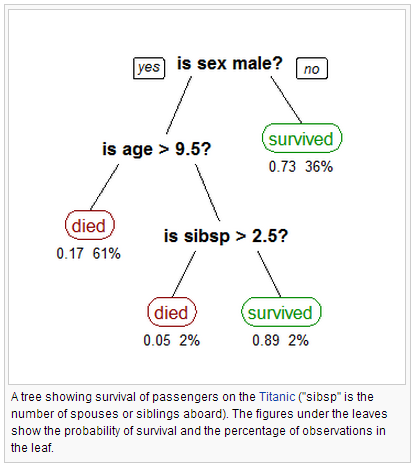
The CART algorithm is structured as a sequence of questions, the answers to which determine what the next question, if any should be.  The result of these questions is a tree like structure where the ends are terminal nodes at which point there are no more questions.  A simple example of a decision tree is as follows [Source: Wikipedia]:

The main elements of CART (and any decision tree algorithm) are:

1. Rules for splitting data at a node based on the value of one variable;
2. Stopping rules for deciding when a branch is terminal and can be split no more; and
3. Finally, a prediction for the target variable in each terminal node.

In order to understand this better, let us consider the Iris dataset (source: UC-Irvine Machine Learning Repository http://archive.ics.uci.edu/ml/).  The dataset consists of 5 variables and 151 records as shown below:

In this data set, "Class" is the target variable while the other four variables are independent variables.  In other words, the "Class" is dependent on the values of the other four variables.  We will use IBM SPSS Modeler v15 to build our tree.  To do this, we attach the CART node to the data set.  Next, we choose our options in building out our tree as follows:

On this screen, we pick the maximum tree depth, which is the most number of "levels" we want in the decision tree.  We also choose the option of "Pruning" the tree which is used to avoid over-fitting.  More about pruning in a different blog post.

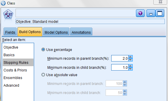
On this screen, we choose stopping rules, which determine when further splitting of a node stops or when further splitting is not possible.  In addition to maximum tree depth discussed above, stopping rules typically include reaching a certain minimum number of cases in a node, reaching a maximum number of nodes in the tree, etc.  Conditions under which further splitting is impossible include when [Source: Handbook of Statistical Analysis and Data Mining Applications by Nisbet et al]:

• Only one case is left in a node;
• All other cases are duplicates of each other; and
• The node is pure (all target values agree).

Next we run the CART node and examine the results.  We first look at Predictor Importance, which represents the most important variables used in splitting the tree:

From the chart above, we note that the most important predictor (by a long distance) is the length of the Petal followed by the width of the Petal.

A scatter plot of the data by plotting Petal length by Petal width also reflects the predictor importance:

This should also be reflected in the decision tree generated by the CART.  Let us examine this next:

As can be seen, the first node is split based on our most important predictor, the length of the Petal.  The question posed is "Is the length of the petal greater than 2.45 cms?".  If not, then the class in which the Iris falls is "setosa".  If yes, then the class could be either "versicolor" or "virginica".  Since we have completely classified "setosa" in Node 1, that becomes a terminal node and no additional questions are posed there.  However, we still need to Node 2 still needs to be broken down to separate out "versicolor" and "virginica". Therefore, the next question needs to be posed which is based on our second most important predictor, the width of the Petal.

As expected, in this case, the question relates to the width of the Petal.  From the nodes, we can see that by asking the second question, the decision tree has almost completely split the data separately into "versicolor" and "virginica".  We can continue splitting them further until there is no overlap between classes in each node; however, for the purposes of this post, we will stop our decision tree here.  We attach an Analysis node to see the overall accuracy of our predictions:

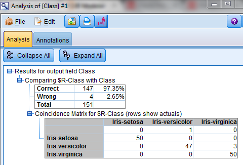
From the analysis, we can see that the CART algorithm has classified "setosa" and "virginica" accurately in all cases and accurately classified "versicolor" in 47 of the 50 cases giving us an overall accuracy of 97.35%.

Some useful features and advantages of CART [adapted from: Handbook of Statistical Analysis and Data Mining Applications by Nisbet et al]:

• CART is nonparametric and therefore does not rely on data belonging to a particular type of distribution.
• CART is not significantly impacted by outliers in the input variables.
• You can relax stopping rules to "overgrow" decision trees and then prune back the tree to the optimal size.  This approach minimizes the probability that important structure in the data set will be overlooked by stopping too soon.
• CART incorporates both testing with a test data set and cross-validation to assess the goodness of fit more accurately.
• CART can use the same variables more than once in different parts of the tree.  This capability can uncover complex interdependencies between sets of variables.
• CART can be used in conjunction with other prediction methods to select the input set of variables.