Predictive maintenance
Machinery and equipment are typically serviced on a scheduled basis, determined either by the time lapsed since the last service or by the usage since the last service. But is this the most effective way to service equipment? If despite regular servicing, a machine fails, then costs associated with unscheduled failure are incurred. And even if machines do not fail on a unscheduled basis, costs incurred on regular, scheduled maintenance may be more than necessary.
To explain this further, let us use an example. Let us take the case of a simple machine that has three components A, B and C. Let's say part A has a life of 3 months, part B has a life of 4 months and part C has a life of 5 months. In order for the machine to keep functioning, we would need to replace part A every 3 months, part B every 4 months and so on. This would mean that after the first three months, we would need to bring the machine down every month to replace at least one part! In order to avoid this, one approach would be replace all three parts on a 3 month cycle. While this would avoid monthly maintenance, it would increase costs on components B and C which would be discarded before their useful lives. Things could get even more complicated if environmental reasons impacted the useful lives of these components. If there was a fluctuation in electricity or temperature and that reduced the life of a component, there will likely be an unscheduled failure which would further increase costs. Also, the interaction between the three components would have an impact on their useful lives. As you can appreciate, there are several factors at play in a simple machine with just 3 components. In larger machines, the level complexity is exponentially greater.
What if there was a way to service a machine at just the right time? With predictive analytics this is possible. In today's post, we will focus on condition monitoring. So what is condition monitoring? Per Wikipedia, condition monitoring is the process of monitoring a parameter of condition in machinery, such that a significant change is indicative of a developing failure. It is a major component of predictive maintenance. The use of conditional monitoring allows maintenance to be scheduled, or other actions to be taken to avoid the consequences of failure, before the failure occurs. Nevertheless, a deviation from a reference value (e.g. temperature or vibration behavior) must occur to identify impeding damages. Predictive maintenance does not predict failure. Machines with defects are more at risk of failure than defect free machines. Once a defect has been identified, the failure process has already commenced and condition monitoring systems can only measure the deterioration of the condition. Intervention in the early stages of deterioration is usually much more cost effective than allowing the machinery to fail. Condition monitoring has a unique benefit in that the actual load, and subsequent heat dissipation that represents normal service can be seen and conditions that would shorten normal lifespan can be addressed before repeated failures occur.
Let us turn our attention now to building a model in SPSS Modeler for condition monitoring. For this purpose, we will use the data contained in the demos folder of SPSS Modeler. [Note: This file is being used for informational / educational purposes only. If using this file infringes on anyone's copyrights, please let me know via the comments section and I will delete all references to this file in this post.]
We first start by examining the data. We add a table node to the source node and execute the table node. The results are as follows:
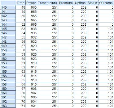
We have the following fields in the data:
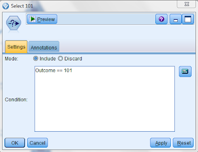
In order to examine the data further, we add a select node to the source node and select those records where the outcome = 101 as follows:
We do the same for outcomes 202 and 303 as well. We then attach two plot nodes to each of the three select nodes and plot the following values:
The plots display as follows:
Time versus temperature for outcome 101:
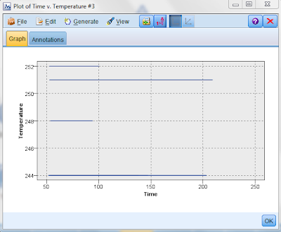
From the above, we can conclude the following:
1) Outcome 101 occurs even though there is no fluctuation in temperature
2) The equipment lasts longest at temperature 251 or 244 where as it fails pretty quickly at 248 and 252.
Time versus temperature for outcome 202:


From the above it is clear that there are similarities in 101 and 303 errors while 202 errors are different. Let us now review the time versus power charts to see if we observe similar results there.
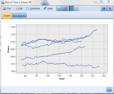
Time versus power for outcome 101:

We observe for outcome 101, that power reduces over time.
Time versus power for outcome 202:
For outcome 202, we observe that power fluctuates widely.
Time versus power for outcome 303:

We observe for outcome 303, that power reduces over time.
Once again, it is clear that there are similarities in 101 and 303 errors while 202 errors are different. Based on these charts it is also clear that the rate of change of temperature and pressure as well as the fluctuation in temperature and pressure play are role in determining which type of errors occur. Therefore, in our analysis, we should include measures for these attributes.
We are now ready to commence modeling. We first add a derive node to create a new field that counts the number of pressure warnings. This field resets when time = 0:

Next, we add another derive node to calculate the rate of change of temperature over time as follows:

The @DIFF1 function returns the first differential of Temperature with respect to Time. This is calculated as follows:
{(Temperature at time n+1) - (Temperature at n)} / {(Time at n+1) - (Time at n)}
In other words, this node derives a field that calculates the rate of change of temperature over time.
The next node we add is another derive node to calculate the rate of change of power over time (this is very similar to the previous derive node to that calculates the rate of change of temperature over time).
Next, we add another derive node to determine whether the power is fluctuating or not. A power flux is true if power varies in different directions between record n and record (n - 1). In order to determine this, we create a flag in the derive node as follows:

The @OFFSET formula returns the value of field (PowerInc) in the record offset from the current record by the value of expression (1).
We then derive the power state which is another flag. The power state starts of as Stable but is designated as Fluctuating when two successive power fluxes are detected. It switches back to Stable when there has not been a power flux for five time intervals or when the time is reset. This is achieved as follows:

The @SINCE command returns the number of records that have passed since the expression was true, not considering the current record.
We add another derive node to calculate the power change which is the average of PowerInc over the last five intervals. This is achieved as follows:

We perform a similar calculation for temperature change using another derive node.
So far, the modeling stream appears as follows:

To examine what the data looks like after making these changes, we add a table node to the last derive node and execute the node. The results are as follows:

We then attach a select node to discard the first record of each time series to avoid large, unnatural jumps in power and temperature. This is achieved as follows:

We then attach a filter node to discard the initial fields and retain the derived fields as follows:

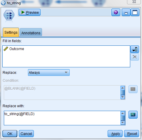
We then add two filler nodes, one to convert all values in the Outcome field to a String measurement type and the other to convert the Pressure Warnings field to a Number measurement type as follows:


We are now ready to create our modeling nugget. To do this, we add a type node and identify the Outcome filed as the target field as follows:

We then attach a C5 node to the type node and execute it to generate our modeling nugget. We then attach an analysis node and observe the following results:

On comparing the predicted results with the observed results, we observe that the model has 99.79% accuracy.
To explain this further, let us use an example. Let us take the case of a simple machine that has three components A, B and C. Let's say part A has a life of 3 months, part B has a life of 4 months and part C has a life of 5 months. In order for the machine to keep functioning, we would need to replace part A every 3 months, part B every 4 months and so on. This would mean that after the first three months, we would need to bring the machine down every month to replace at least one part! In order to avoid this, one approach would be replace all three parts on a 3 month cycle. While this would avoid monthly maintenance, it would increase costs on components B and C which would be discarded before their useful lives. Things could get even more complicated if environmental reasons impacted the useful lives of these components. If there was a fluctuation in electricity or temperature and that reduced the life of a component, there will likely be an unscheduled failure which would further increase costs. Also, the interaction between the three components would have an impact on their useful lives. As you can appreciate, there are several factors at play in a simple machine with just 3 components. In larger machines, the level complexity is exponentially greater.
What if there was a way to service a machine at just the right time? With predictive analytics this is possible. In today's post, we will focus on condition monitoring. So what is condition monitoring? Per Wikipedia, condition monitoring is the process of monitoring a parameter of condition in machinery, such that a significant change is indicative of a developing failure. It is a major component of predictive maintenance. The use of conditional monitoring allows maintenance to be scheduled, or other actions to be taken to avoid the consequences of failure, before the failure occurs. Nevertheless, a deviation from a reference value (e.g. temperature or vibration behavior) must occur to identify impeding damages. Predictive maintenance does not predict failure. Machines with defects are more at risk of failure than defect free machines. Once a defect has been identified, the failure process has already commenced and condition monitoring systems can only measure the deterioration of the condition. Intervention in the early stages of deterioration is usually much more cost effective than allowing the machinery to fail. Condition monitoring has a unique benefit in that the actual load, and subsequent heat dissipation that represents normal service can be seen and conditions that would shorten normal lifespan can be addressed before repeated failures occur.
Let us turn our attention now to building a model in SPSS Modeler for condition monitoring. For this purpose, we will use the data contained in the demos folder of SPSS Modeler. [Note: This file is being used for informational / educational purposes only. If using this file infringes on anyone's copyrights, please let me know via the comments section and I will delete all references to this file in this post.]
We first start by examining the data. We add a table node to the source node and execute the table node. The results are as follows:

We have the following fields in the data:
- Time
- Power
- Temperature
- Pressure warning (0 = normal; 1 = warning)
- Uptime (time elapsed since last service)
- Error status (Normal = 0; Error = 101, 202 or 303)
- Outcome - this is available only with the benefit of hindsight. This field indicates an error (101, 202 or 303) when a "period leading to a fault" commences and returns to normal (0) when the equipment is repaired and the time is reset.
In order to examine the data further, we add a select node to the source node and select those records where the outcome = 101 as follows:

We do the same for outcomes 202 and 303 as well. We then attach two plot nodes to each of the three select nodes and plot the following values:
- Time versus temperature
- Time versus power
The plots display as follows:
Time versus temperature for outcome 101:
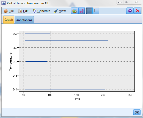
From the above, we can conclude the following:
1) Outcome 101 occurs even though there is no fluctuation in temperature
2) The equipment lasts longest at temperature 251 or 244 where as it fails pretty quickly at 248 and 252.
Time versus temperature for outcome 202:

From the above, we can conclude the following:
1) Outcome 202 occurs even when there is a steady rise in temperature over time
2) The equipment fails with a 202 error almost as soon as the temperature hits 320.
Time versus temperature for outcome 303:

From the above, we can conclude the following:
1) Outcome 303 occurs even though there is no fluctuation in temperature
2) The equipment lasts longest at temperature 248 or 258 where as it fails pretty quickly at 250, 255 or below 245.
From the above it is clear that there are similarities in 101 and 303 errors while 202 errors are different. Let us now review the time versus power charts to see if we observe similar results there.
Time versus power for outcome 101:

We observe for outcome 101, that power reduces over time.
Time versus power for outcome 202:

For outcome 202, we observe that power fluctuates widely.
Time versus power for outcome 303:

We observe for outcome 303, that power reduces over time.
Once again, it is clear that there are similarities in 101 and 303 errors while 202 errors are different. Based on these charts it is also clear that the rate of change of temperature and pressure as well as the fluctuation in temperature and pressure play are role in determining which type of errors occur. Therefore, in our analysis, we should include measures for these attributes.
We are now ready to commence modeling. We first add a derive node to create a new field that counts the number of pressure warnings. This field resets when time = 0:

Next, we add another derive node to calculate the rate of change of temperature over time as follows:

The @DIFF1 function returns the first differential of Temperature with respect to Time. This is calculated as follows:
{(Temperature at time n+1) - (Temperature at n)} / {(Time at n+1) - (Time at n)}
In other words, this node derives a field that calculates the rate of change of temperature over time.
The next node we add is another derive node to calculate the rate of change of power over time (this is very similar to the previous derive node to that calculates the rate of change of temperature over time).
Next, we add another derive node to determine whether the power is fluctuating or not. A power flux is true if power varies in different directions between record n and record (n - 1). In order to determine this, we create a flag in the derive node as follows:

The @OFFSET formula returns the value of field (PowerInc) in the record offset from the current record by the value of expression (1).
We then derive the power state which is another flag. The power state starts of as Stable but is designated as Fluctuating when two successive power fluxes are detected. It switches back to Stable when there has not been a power flux for five time intervals or when the time is reset. This is achieved as follows:

The @SINCE command returns the number of records that have passed since the expression was true, not considering the current record.
We add another derive node to calculate the power change which is the average of PowerInc over the last five intervals. This is achieved as follows:

We perform a similar calculation for temperature change using another derive node.
So far, the modeling stream appears as follows:

To examine what the data looks like after making these changes, we add a table node to the last derive node and execute the node. The results are as follows:

We then attach a select node to discard the first record of each time series to avoid large, unnatural jumps in power and temperature. This is achieved as follows:

We then attach a filter node to discard the initial fields and retain the derived fields as follows:

We then add two filler nodes, one to convert all values in the Outcome field to a String measurement type and the other to convert the Pressure Warnings field to a Number measurement type as follows:

We are now ready to create our modeling nugget. To do this, we add a type node and identify the Outcome filed as the target field as follows:

We then attach a C5 node to the type node and execute it to generate our modeling nugget. We then attach an analysis node and observe the following results:

On comparing the predicted results with the observed results, we observe that the model has 99.79% accuracy.


Thanks for sharing! This page was very informative and I enjoyed it. Predictive maintenance
ReplyDeleteThank you.
Delete