Creating a time series forecast using IBM SPSS Modeler
In today's post, we discuss how to create a time series forecast using IBM SPSS Modeler. For the purposes of our exercise, we will use historical sales data at a SKU (stock keeping unit) level. This data is provided in a MicroSoft Excel .xlsx file and must be in the following format:
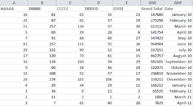
In the image above, AAAAA through EEEEE are SKU numbers with the relevant monthly sales data provided in the respective columns. There is also a column that indicates the grand total of all SKUs sold in a month (AAAAA +...+ EEEEE + other SKUs not shown in the image above). The last column in the image above reflects the months for which historical sales data are provided.
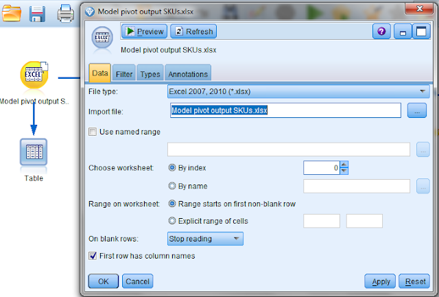
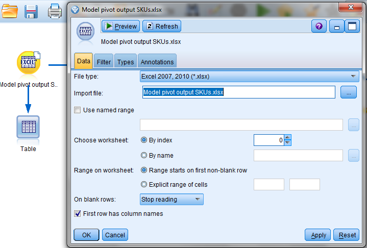
As with any modeling exercise, we first insert a source node into the modeling canvas. Since our data is in the MicroSoft Excel .xlsx file format, we insert an Excel source node as follows:
On exporting to a Table node, we see the output display as follows:

We then add a Filter node to select the five SKUs that we will be creating the time series forecast for:

We then add a Type node to identify the measurement type of each of Field and assign Roles to each field. Note from the image below that all fields here are assigned the role of "Target" since we want to forecast values for each of these fields. The date field is assigned the role "None":

Since the date format does not appear to be correct, we insert a reclassify node to create a new field called Date_New as follows:

The output now appears as follows:

As can be seen above, the new date field with the correct format appears next to the old field with the incorrect format. We then add a filter node to filter out the old date field with the incorrect format as follows:

We then add another Type node to assign the "None" role to the new date field as follows:

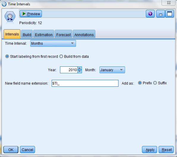
We then add a Time Intervals node from the Field Ops tab:

The Time Intervals node allows you to specify intervals and generate labels for time series data to be used in a Time Series modeling or a Time Plot node for estimating or forecasting. A full range of time intervals is supported, from seconds to years. For example, if you have a series with daily measurements beginning January 3, 2005, you can label records starting on that date, with the second row being January 4, and so on. You can also specify the periodicity—for example, five days per week or eight hours per day (IBM SPSS Modeler Help).
The time interval node is used to specified specify intervals as follows:

Before we insert the Time Series modeling node, there is one last action that needs to be taken with respect to the Time Interval node. This is in the Forecast tab of the Time Intervals node where we tick the "Extend records into the future" box and choose the number of months for which we want to create the forecast for:

We are now ready to insert the Time Series modeling node into the modeling canvas and attach it to the Time Intervals node. We choose the default options as follows and Run the node:

Finally, we attach a Time Plot node to the modeling nugget and evaluate the results:

As can be seen from the above time plot, the model has created a forecast for SKU ID AAAAA extending the historical sales numbers by the specified 6 months.
http://bluelineplanning.com

In the image above, AAAAA through EEEEE are SKU numbers with the relevant monthly sales data provided in the respective columns. There is also a column that indicates the grand total of all SKUs sold in a month (AAAAA +...+ EEEEE + other SKUs not shown in the image above). The last column in the image above reflects the months for which historical sales data are provided.
As with any modeling exercise, we first insert a source node into the modeling canvas. Since our data is in the MicroSoft Excel .xlsx file format, we insert an Excel source node as follows:
On exporting to a Table node, we see the output display as follows:

We then add a Filter node to select the five SKUs that we will be creating the time series forecast for:

We then add a Type node to identify the measurement type of each of Field and assign Roles to each field. Note from the image below that all fields here are assigned the role of "Target" since we want to forecast values for each of these fields. The date field is assigned the role "None":

Since the date format does not appear to be correct, we insert a reclassify node to create a new field called Date_New as follows:

The output now appears as follows:

As can be seen above, the new date field with the correct format appears next to the old field with the incorrect format. We then add a filter node to filter out the old date field with the incorrect format as follows:

We then add another Type node to assign the "None" role to the new date field as follows:

We then add a Time Intervals node from the Field Ops tab:
The Time Intervals node allows you to specify intervals and generate labels for time series data to be used in a Time Series modeling or a Time Plot node for estimating or forecasting. A full range of time intervals is supported, from seconds to years. For example, if you have a series with daily measurements beginning January 3, 2005, you can label records starting on that date, with the second row being January 4, and so on. You can also specify the periodicity—for example, five days per week or eight hours per day (IBM SPSS Modeler Help).
The time interval node is used to specified specify intervals as follows:
Before we insert the Time Series modeling node, there is one last action that needs to be taken with respect to the Time Interval node. This is in the Forecast tab of the Time Intervals node where we tick the "Extend records into the future" box and choose the number of months for which we want to create the forecast for:

We are now ready to insert the Time Series modeling node into the modeling canvas and attach it to the Time Intervals node. We choose the default options as follows and Run the node:

Finally, we attach a Time Plot node to the modeling nugget and evaluate the results:

As can be seen from the above time plot, the model has created a forecast for SKU ID AAAAA extending the historical sales numbers by the specified 6 months.
http://bluelineplanning.com


thanks, SPSS is a good data analysis tool for us.
ReplyDeleteHi Venky, thanks for such a nice explanation of time series model. But I have a question, what operations shall we apply on the data if it has seasonality/unseasonality ? How to transform the data ? Because I'm facing a problem with the same issue, due to which the predictions are not coming properly. I'll appreciate your help for the same. Thanks in advance.
ReplyDeleteHi Pankaj, please review my latest video blog on time series forecasting techniques. Hopefully that will answer you r question. The Expert Modeler feature in SPSS Modeler will also help. Thanks for your comment.
Deletesecond day is imparted for the good and waves of the world. It has been sharply followed for the visits of the spss expert for all issues. The tangible item has been highlighted for the success of the citizens.
ReplyDeleteA student was struggling to create a time series forecast using IBM SPSS Modeler for their data analysis assignment. The software seemed complex, and the student wasn’t sure how to choose the right model. With the deadline approaching, the student decided to seek help from a reliable service offering buy assignment UK the experts helped the student understand how to use SPSS Modeler effectively, ensuring they could complete the assignment successfully. This experience showed how getting support when needed can make a big difference in finishing assignments on time.
ReplyDeleteSPSS is one of the most powerful tools for statistical analysis, often used by students and researchers for data interpretation. While it offers many features, learning to use it effectively can be tricky without proper guidance. For those struggling with data sets, tests, or reports, SPSS assignment help provides expert assistance to simplify concepts, ensure accuracy, and improve academic performance with well-structured solutions.
ReplyDelete