TheMainstreamSeer

 Someone recently asked how to write a Python script that took user input into account and took some action based on the validity of the user input.  Here are some code snippets that I developed for a few different scenarios: 1) A game is being played and it has just ended.  How would you ask the user if they wanted to play again? game_running = True #assuming the game is running play_again = input("Play again? ")  #get user input while True: #restart game if answer is "y" or "Y"         if play_again == 'y' or play_again == "Y":             game_running = True             break         else: #print thank you message and exit the program             print("Thank you for playing!")          ...

This post focuses on dis-aggregated hardware follows my earlier post Open Source Networking: a hierarchical approach .  Hardware dis-aggregation is an important aspect of open networking.  Essentially, dis-aggregated hardware involves software being separated from the underlying hardware.  Similar to a PC or a server where you can boot with a Linux installer CD to Linux, you are able to boot dis-aggregated hardware with an Operating System (OS) installer and install an operating system on it.  Most commercial vendors bundle their hardware with software which means you cannot modify the software or change the OS that it comes loaded with.  Open, dis-aggregated hardware however does not have this restriction. Take for example, Ethernet switches which have two main components: A packet switching/processing ASIC chipset controller A CPU which hosts the software / firmware and the packet switching ASIC. Most commercial vendors bundle the software with their...

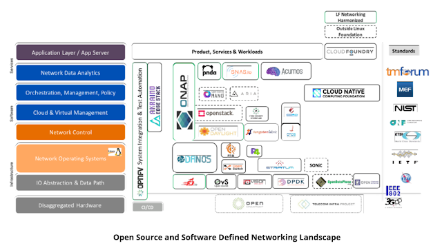
I have been extremely fortunate to be part of several network cloudification projects over the past 18-24 months.  It's been very exciting to see the changes that disaggregation and open source projects have been making to move an industry forward.  Here I capture some initial thoughts about open source networking. Note: while the on-the-job learning has been immense, I have supplemented this with some terrific courses from The Linux Foundation including LinuxFoundationX: LFS165x Introduction to Open Source Networking Technologies by Reza Toghraee. Networking has come a long way from the widespread use of rigid appliances to perform networking functions such as routing, firewalling, switching, and load balancing.  A key principle behind this transformation is disaggregation , i.e. the de-coupling of the software performing the networking functions with the hardware it is installed on.  The main driver of this transformation ...

Are you curious about 5G but not sure what it's all about?  Here's a quick summary to bring you up to speed. A quick refresher about 1G through 4G before we get started: 1G refers to the first generation of wireless cellular technologies that brought us our very first cell phones. 2G was a significant improvement from 1G in the way the radio frequency spectrum was used enabling many more users per frequency band.  Importantly for consumers, 2G enabled digitally encrypted conversations and SMS text messages! 3G was a giant leap forward from 2G.  3G enabled consumers to get online using their cell phones. 4G pushed the limits further with improved speeds and increased applications for consumers including IP telephony, high def mobile TV and video conferencing.  So what does 5G promise?  5G promises to dramatically improve speed, latency and scale. It is expected to be 100X faster than 4G (you could download an HD movie in 1 second!). Its data volume...

There appears to be a lot of confusion between the terms Artificial Intelligence (AI), Machine Learning (ML), Neural Networks (NN) and Deep Learning (DL).  Based on research from various popular blogs and articles, here is my attempt at a simple visual explanation:

To answer interesting questions, you need data. You begin with an observation that you want to understand including anecdotal observations.  For example, a certain website layout attracts more visitors to our web page than a different website layout.  From your observations, you generate explanations or theories of those observations, from which you can make predictions or hypothesis.  To test your hypothesis or predictions, you need data. So you collect relevant data (and to do that you need to identify things that can be measured) and then you analyze those data.  The analysis of your data may support your theory or give you cause to modify the theory. As such, the processes of data collection and analysis and generating theories are intrinsically linked: theories lead to data collection / analysis and data collection / analysis informs theories.  The research process is summarized below: (adapted from Discovering Statistics using R by Andy Field e...

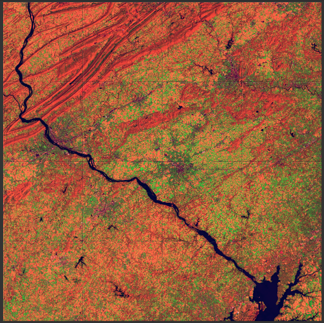
If you are looking for a fun way to experience satellite imagery and learn more about remote sensing, check out Earth Image Puzzles here . Here is a solved jigsaw puzzle of SouthEastern PA: Enjoy!

Courtesy of: Visual Capitalist

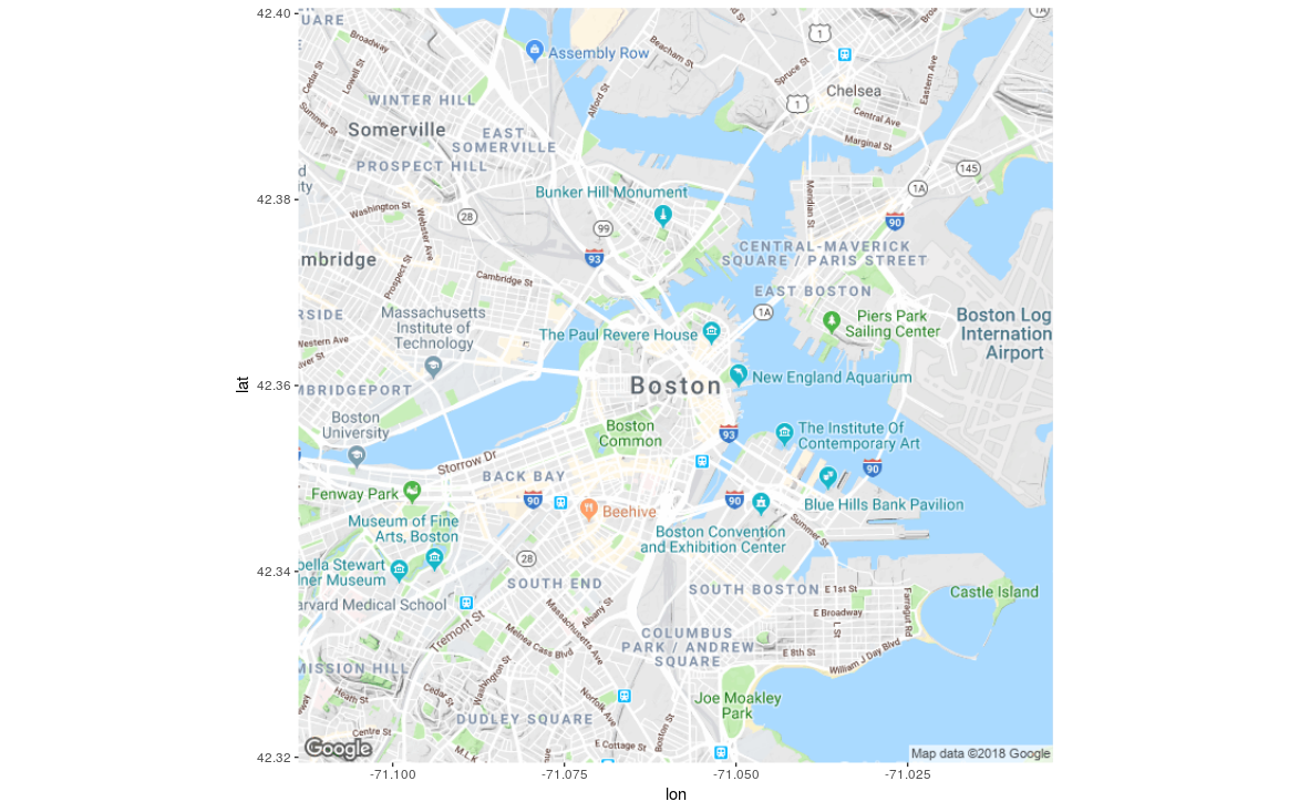
Over the past year, I have been exploring the geospatial capabilities of various R packages.  Today, I want to share the most basic of geospatial capabilities, which is producing a map.  Using R, you can do this in just 5 lines of code. Let's produce a map of Boston, Massachusetts.  Boston has a longitude of -71.0588801 and a latitude of 42.3600825.  Since we list x and y coordinates in order (i.e. we list y after x), we list longitude (the horizontal coordinate) before latitude (the vertical coordinate).  Let's create our map! Code line 1: install.packages("ggmap") This command installs the ggmap package in your R environment. Code line 2: library(ggmap) This command loads the ggmap package in your R environment. Code line 3: boston <- c(lon = -71.0588801, lat = 42.3600825) This line creates a variable called "boston" and assigns the lon and lat coordinates in it. Code line 4: boston_map <- get_map(boston, zoom = 13, scale = 1...

I have the great honor of knowing ex-IBM Fellow Jeff Jonas, the co-Founder, CEO and Chief Scientist of Senzing .  Apart from being exceptionally talented, Jeff is also an amazing human being who is always willing to help others.  I have personally been the beneficiary of his generosity and continue to benefit from his counsel every day.  Jeff is one of the main reasons why I have chosen to follow a technical career path at IBM. Jeff left IBM in 2016 to start a new venture called Senzing .  Senzing has built the first real-time AI software product for Entity Resolution (ER), a space that Jeff is the world's #1 expert in.  Senzing's new offering has huge implications in the post- GDPR world and has the potential to increase trust in Blockchain networks.  Jeff recently gave a keynote at the IBM Think conference where he described what Senzing does and its potential applications (including as part of IBM Blockchain).  I strongly recommend watchin...

This post attempts to visualize the 1854 London Cholera Outbreak based on data collected by Dr. John Snow and provided in the HistData R package. Dr. Snow was able to identify that cholera was a water borne disease by visualizing his data in 1854 and was able to bring the Cholera outbreak to an end. This dataset and analysis speaks to power of geospatial data and its importance in decision making.

The motivation for this blog is to examine the reasons behind the explosion of the USA Space Shuttle Challenger on 28 January, 1986. The night before the launch a decision had to be made regarding launch safety and engineers recommended that the launch be postponed in the event the temperature at launch was below freezing as this adversely impacted the integrity of O-rings, a key component holding in field joints. The engineers advice was ignored and disaster ensued. Let's dive in!

M y  latest publicly available R notebook  created in  IBM's Data Science Experience  is  here !  This notebook provides a tutorial on: This notebook covers: Fitting and interpreting linear models ; Evaluating model assumptions; and Selecting among competing models. I hope you enjoy this  notebook .  Please feel free to share and let me know your thoughts. My latest notebook: Regression in R https://t.co/HDYFzTAFPr #rstats #DataScience #ibmaot #Statistics #Stats #dsx #Bluemix h/t @kabacoff pic.twitter.com/LxKc9HkBC0 — Venky Rao (@VRaoRao) October 15, 2017

If you thought the coefficient of alienation referred to the hostility I receive from my family as I update my blog on a Saturday afternoon, I would not fault you too much.  However, this is a blog about predictive analytics which is based on Statistics.  So let's keep that in mind as we understand what the "Coefficient of Alienation" means. Apart from being one of the coolest sounding Statistical terms, the Coefficient of Alienation measures the proportion of variation in the outcome not “explained” by the variables on the right-hand side of a simple linear regression (ordinary least squares) equation. The Coefficient of Alienation is also known as the Coefficient of Non-Determination since the formula for calculating it is: where: is the Coefficient of Determination. And now before my personal (and non-Statistical) Coefficient of Alienation reaches the point of no return, I will bring this post to an end.

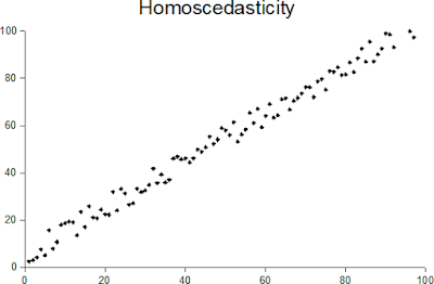
Homoscedasticity and heteroscedasticity - two of the scariest sounding terms in all of Statistics!  So what do they mean? When one calculates the variance or standard deviation of a dataset of random variables, one assumes that the variance is constant across the entire population.  This assumption is homoscedasticity.  The opposite of this assumption is heteroscedasticity. In other words, a collection of random variables is heteroscedastic if there are sub-populations within the dataset that have different variances from others (source: https://en.wikipedia.org/wiki/Heteroscedasticity).  Another way of describing homoscedasticity is constant variance and another way of describing heteroscedasticity is variable variance. Jeremy J Taylor  in his blog  provides a great example of a distribution that is heteroscedastic.  In his example, the independent variable is "age" and the predictor variable is "income".  The example dis...

One of the first things that any student of statistics learns is 2 popular measures of descriptive statistics: mean and standard deviation. Has the approach to calculating Standard Deviation ever got you wondering about the need to square the distances from the mean in order to remove negatives instead of just using the average of the absolute values to eliminate negatives?  Well, you are certainly not alone. As it turns out, squaring the distances from the mean and then calculating their square root to arrive at the Standard Deviation of a distribution is more as a result of convention than anything else.  In fact, there is a measure called the Absolute Mean Deviation that does not take the squared distances from the mean to eliminate negative values.  Instead, it just takes the absolute values of the differences from the mean and calculates the average of the sum of those values to determine deviation from the mean. The convention of course is to use ...

M y  latest publicly available R notebook  created in  IBM's Data Science Experience  is  here !  This notebook provides a tutorial on: This notebook covers: Descriptive statistics Frequency and contingency tables Correlations and covariances t-tests; and Nonparametric statistics. I hope you enjoy this  notebook .  Please feel free to share and let me know your thoughts. My latest R notebook: Basic #Statistics in R https://t.co/b3NmhNXI5X #DataScience #dsx #IBM #Bluemix #ibmaot #rstats h/t @kabacoff pic.twitter.com/AsIhr51Q5l — Venky Rao (@VRaoRao) September 13, 2017